Pick the model by token profile, not by benchmarks alone
A benchmark tells you which capability tier a model belongs to. It cannot tell you what that model will cost on your work. This piece is about the second axis, and the map it produces.
Every team I work with asks some version of the same question: which model should we use for this? For two years the honest answer was to point at a leaderboard. That answer was never complete, and in 2026 it stopped being sufficient on its own, not because leaderboards got worse but because they got harder to compare while the cost of getting the choice wrong grew by an order of magnitude.
There are really two questions hiding inside the one being asked. Is this model good enough for the task? is a capability question, and benchmarks, plus your own evaluations, are how you answer it. What will this model cost on this particular kind of work? is an economic question, and no leaderboard answers it, because the answer depends on the shape of your work rather than on the model.
Use only the first axis and you get the two failure modes I see most often: teams running a frontier model on ticket triage because “classification is delicate”, and teams running an underpowered model on work that never closes on the first attempt, paying twice in retries. This piece is about the second axis: cluster the work by token profile, and once the capability question is settled, the cost question mostly answers itself.
What benchmarks stopped telling us
The first axis is still necessary, but it narrowed. Three things happened in the space of a few months.
OpenAI retired SWE-bench Verified in February 2026. Their stated reasons are worth reading in full: 59.4% of the audited problems have broken test cases that reject functionally correct solutions, and the set is contaminated by training data to the point that frontier models reproduce the original human fix. The audit covered 27.6% of the dataset and was weighted towards the problems models failed most often, so the figure is not a claim about the whole set. It does not need to be. Google stopped publishing SWE-bench Verified, GPQA, AIME and MMLU-Pro for Gemini 3.5 and later. Artificial Analysis dropped GPQA Diamond from its index for saturation. So the four numbers most comparison tables were built on are no longer maintained by the people who made those tables meaningful.
Then there is the scaffold problem, which is worse because it looks like it isn’t there. On SWE-bench Pro, Claude Opus 4.6 scores 51.9% under Scale AI’s standardised harness. Vendor-reported figures for comparable models run up to 80%. That is a 28-point gap produced by the harness, not the model. On Terminal-Bench 4.0 the models run inside different agents: GPT-6 Astra under Codex, the Claude models under Claude Code. Those rows are not a model-versus-model comparison at all, and they mix model generations besides. An agentic benchmark measures the pair.
And a practical annoyance: the official leaderboards for SWE-bench, LiveBench, Terminal-Bench and ARC Prize render their rows in JavaScript. Most of the numbers circulating today come from aggregators quoting each other, and the aggregators disagree. I found the same model priced at $0.96 per million tokens by one source and $0.10 by another, nearly a factor of ten, and nobody reconciles it.
None of this makes benchmarks useless, and I am not proposing to drop them. They still do the job nothing else does: they place a model in a capability tier and they rule models out. What they no longer do reliably is discriminate within a tier, and they never did tell you what a model would cost on your work. That is the gap the second axis fills.
The second axis: the token profile
Here is the part that changed how I think about it.
The instinct is to group work by discipline: development, analysis, support. That produces clusters that behave nothing alike in production. Take “development”. Reverse engineering an undocumented legacy component means reading an enormous amount of code and writing a few pages of documentation: roughly 135,000 tokens in, 5,500 out, with 17% of the cost coming from the output. Greenfield development is the mirror image: a small amount of context, a lot of generated code, roughly 40,000 in and 12,000 out, with 60% of the cost coming from the output. Same discipline, same team, same week. Opposite economics.
That difference is not cosmetic, because it decides which lever works. The input-dominated cluster is a caching and retrieval problem, and it is the only kind of work where the vendor’s long-context pricing changes the ranking. The output-dominated cluster is an effort and response-length problem, where reasoning tokens are billed as output at all three major vendors. Average the two into one “development” row and you get a number that describes neither, plus a recommendation that is wrong for both.
Group by token profile instead and the clusters come out homogeneous, and each one becomes a question a benchmark cannot answer but arithmetic can. Thirteen of them cover most of what a software organisation does:
| Family | Cluster | Input (range) | Output (range) | Cost from output |
|---|---|---|---|---|
| Analysis and documentation | Requirements analysis | 15,000 (6k–40k) | 3,000 (1.5k–6k) | 50% |
| Documentation and reverse engineering | 135,000 (40k–400k) | 5,500 (2k–12k) | 17% | |
| Regulatory analysis | 30,000 (10k–90k) | 1,500 (0.8k–4k) | 20% | |
| Development | Greenfield development | 40,000 (15k–100k) | 12,000 (5k–30k) | 60% |
| Maintenance on existing code | 60,000 (25k–150k) | 4,500 (2k–12k) | 27% | |
| Technology migration | 90,000 (40k–250k) | 9,000 (4k–25k) | 33% | |
| Data | Data handling and ETL | 20,000 (8k–60k) | 4,000 (1.5k–12k) | 50% |
| Quality | Code review | 25,000 (8k–70k) | 1,500 (0.6k–4k) | 23% |
| Test generation | 20,000 (8k–50k) | 5,000 (2k–15k) | 56% | |
| Operations and support | Application operations | 60,000 (15k–200k) | 2,000 (0.8k–6k) | 14% |
| Ticket triage | 2,000 (0.8k–6k) | 150 (60–500) | 27% | |
| Document extraction | 6,000 (2k–25k) | 500 (200–2k) | 29% | |
| Operator assistance | 5,000 (1.5k–20k) | 500 (200–2k) | 33% |
The central figures are working assumptions, not measurements, and the ranges are there on purpose: a single number would claim a precision nobody has. For documentation and reverse engineering the plausible input runs from 40,000 to 400,000 tokens depending entirely on whether you analyse one module or the whole repository, and locating yourself inside that range is the first piece of work. The cost share assumes the 5x output-to-input ratio common to the proprietary models. That assumption is load-bearing, because the share is what picks the lever. Recompute it at the 1.3x of Qwen3.8-27B and greenfield falls from 60% to 28%, test generation from 56% to 25%, requirements analysis from 50% to 21%. On an open-weight model, in other words, several clusters stop being output problems and become input problems, and the lever to pull first changes with them. The column below is the proprietary case; if you are running open weights, halve it and read again. Replace the centres with the medians from your own logs as soon as you have two weeks of them. Changing them moves the distances; it does not change the ordering.
The map
Once the clusters are defined, the model question becomes arithmetic. Take each cluster’s token profile, apply it to each model’s list price, and you get what that model actually costs for that kind of work.
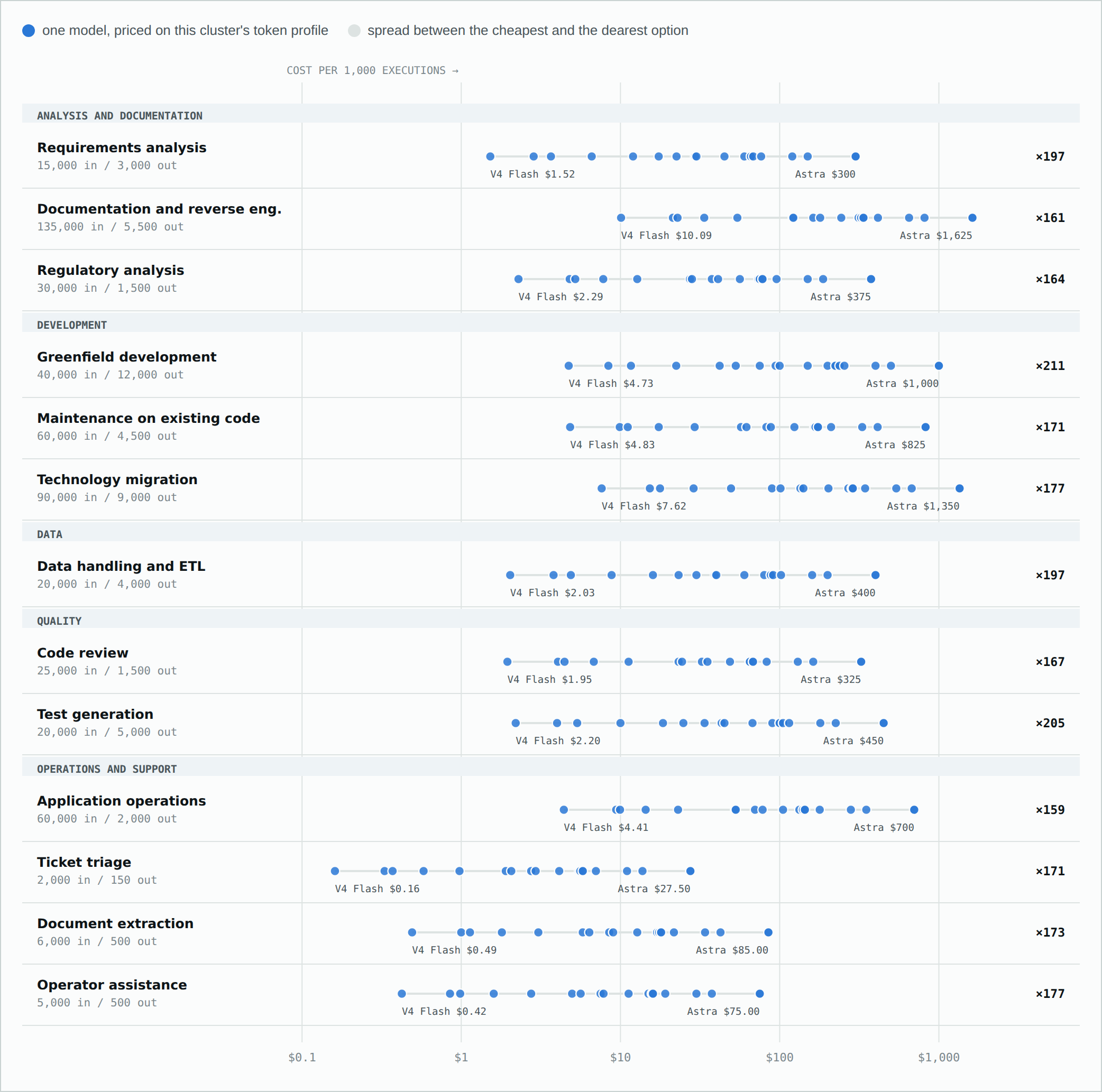
Two distances matter here, and neither is visible from a price list.
The distance within a row is the decision. In ticket triage the range across the models on the market runs from $0.161 to $27.50 per thousand executions, a factor of 171 on the same task. Every row has a spread of that order, between 159x and 211x. No public evidence says the expensive model classifies your tickets better. A factor like that has to be justified by a measurement, not by caution, and in my experience it usually cannot be.
The distance between rows is the budget. The same Gemini 3.8 Flash costs $2.06 per thousand triage calls and $121.88 per thousand legacy-documentation runs. Fifty-nine times the bill, same model, same price per token. Anyone sizing a project from the per-token list price alone is off by an order of magnitude before they start.
There is also a floor effect worth naming. In triage, extraction and operator assistance the difference between all the reasonable options is a few dollars a month at normal volume. Optimising there is a waste of engineering time: choose for quality and latency instead. Real cost optimisation lives in the development family and in legacy documentation, where a bad choice gets multiplied by the volume of context.
The profile decides the lever
The same reframe answers the second question teams ask, which is what to do about the bill.
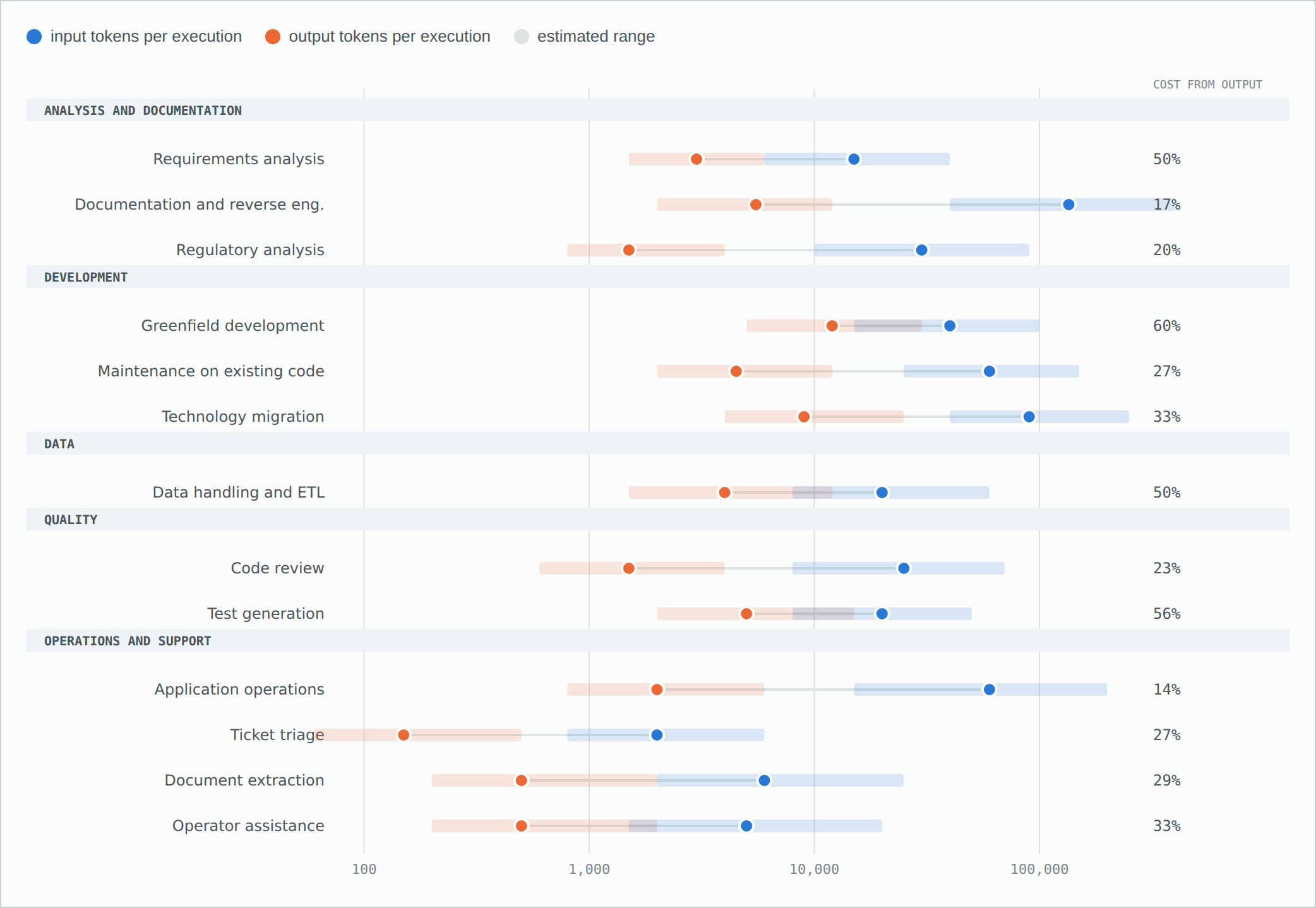
The spread on the right-hand column is the actionable part: 14% for application operations, 60% for greenfield. That is the difference between a problem you solve with a cache and a problem you solve with an effort setting.
It also puts a ceiling on what optimisation can return. Apply the levers that suit a cluster’s profile and the saving comes out around 68% on ticket triage and 15% on greenfield development. Those two figures are my arithmetic, not a vendor’s: they assume the vendors’ declared rates in the chart below, a cache reuse of 70% of the input in the clusters with a stable prefix and 45% where it is partial, and batch on the clusters that can wait. What is striking is that they barely move with the model you picked. The ceiling is set by the profile, not by the price list: in greenfield the money is in the output, and caching does not touch it. In input-heavy clusters the fix is configuration; in output-heavy clusters it is changing how you work, generating in increments and calibrating effort.
| Cluster | Prefix cache | Batch | Effort and output | Retrieval | Tool search | Distillation |
|---|---|---|---|---|---|---|
| Requirements analysis | medium | low | high | medium | – | – |
| Documentation and reverse engineering | high | medium | low | high | medium | – |
| Regulatory analysis | high | medium | medium | high | low | – |
| Greenfield development | medium | – | high | low | medium | – |
| Maintenance on existing code | high | – | medium | medium | high | – |
| Technology migration | high | low | high | medium | high | – |
| Data handling and ETL | medium | high | medium | low | low | medium |
| Code review | high | medium | low | medium | low | – |
| Test generation | medium | high | high | low | low | low |
| Application operations | high | low | medium | high | medium | – |
| Ticket triage | high | high | low | – | – | high |
| Document extraction | medium | high | low | – | – | high |
| Operator assistance | high | – | medium | medium | low | – |
What each lever is actually worth
These are the reductions the vendors themselves publish, including a few levers narrower than the six in the table above. I have not verified any of them independently, and they are not additive: each acts on a different base.
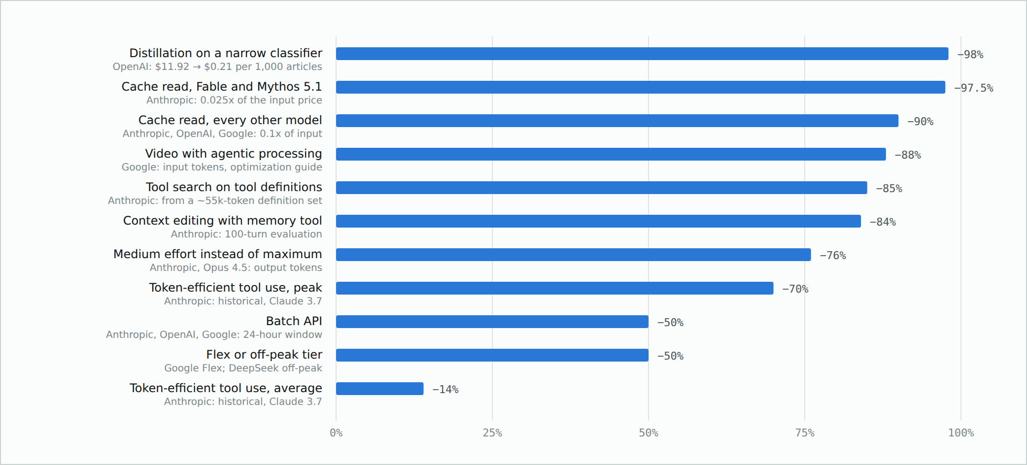
Three of them deserve a note.
Caching is the biggest lever and the most misunderstood. A cache read costs a tenth of the input price at all three vendors, with one exception visible in the chart: Anthropic prices cache reads on Fable and Mythos 5.1 at 0.025x, a fortieth. The write, on the other hand, costs 1.25x, or 2x for Anthropic’s one-hour cache. Anthropic states break-even after a single read on the five-minute cache and two reads on the one-hour cache. It needs a stable prefix: the minimum cacheable block runs from 512 to 4,096 tokens on Anthropic depending on the model, 1,024 on OpenAI from GPT-5.6 onward, 4,096 on the Gemini 3.x line. Changing your tool definitions, your images or your thinking parameters invalidates it. Anthropic reports observed hit rates between 30% and 98%, and the distance between those two numbers is the entire business case.
Batch is half price on everything that is not interactive, at all three vendors, with a declared 24-hour window. Anthropic says the batch discount stacks with caching; Google bills cache hits at the caching rate rather than the batch rate. In the table above, four of the thirteen clusters are natural batch candidates: test generation, ETL, triage and extraction. Most teams simply never switch it on.
Distillation is the only order-of-magnitude jump. OpenAI’s published example on a classifier: $11.92 per thousand articles with the large model few-shot, $0.21 with a small model fine-tuned on a thousand labelled examples, at the same stated 91.5% accuracy. Under 2% of the cost. It only works on narrow, stable tasks, which in this taxonomy means triage and document extraction.
Two levers that look like savings and are not always: Anthropic’s server-side compaction is an extra sampling step that gets billed and does not appear in the top-level counters, so you have to sum usage.iterations; and context editing invalidates cached prefixes and forces new writes, which is what the clear_at_least parameter exists for. Both pay off on long sessions, which in practice means the development and migration clusters, not short repeated calls.
The price list, and one caveat that undoes it
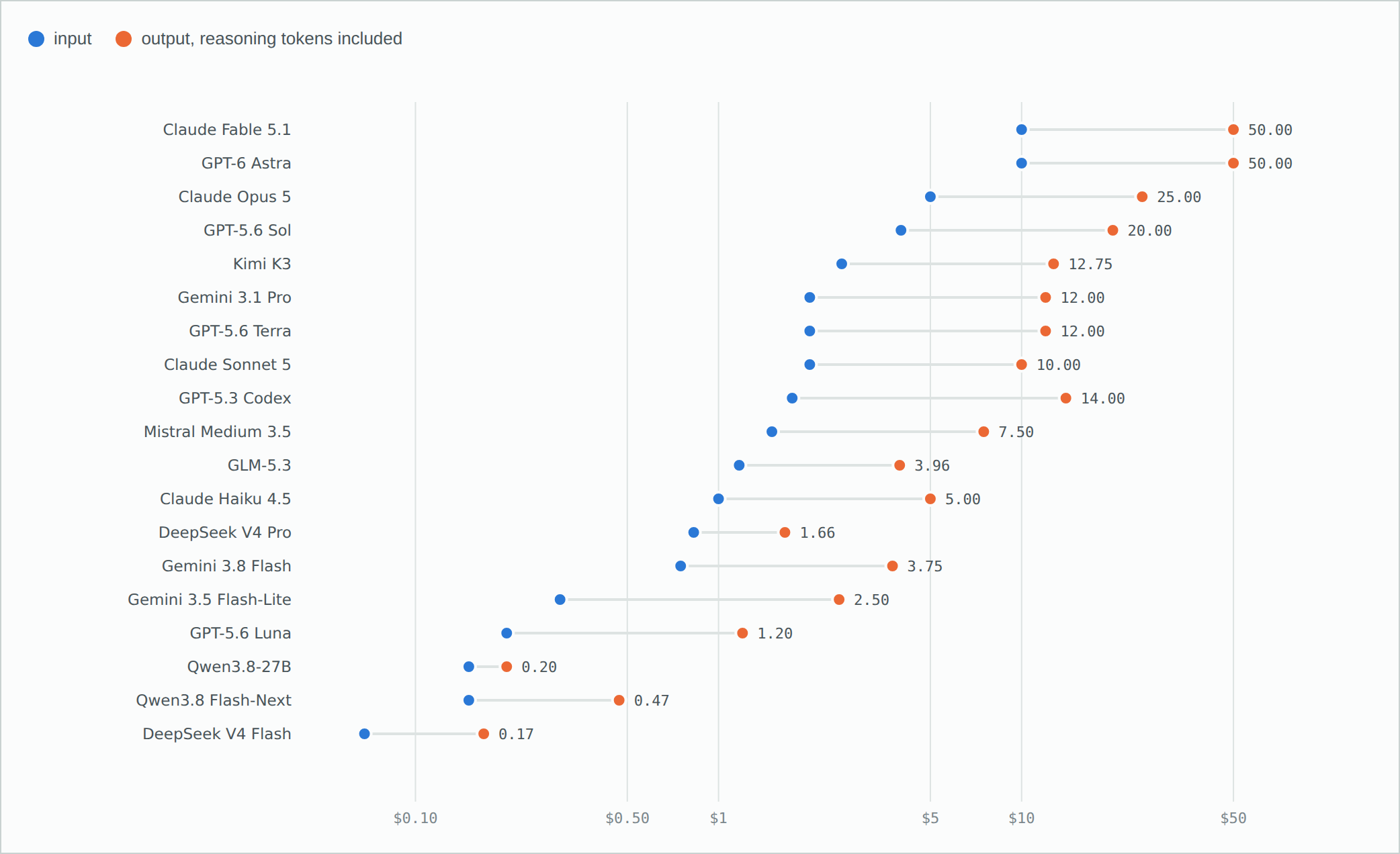
The output-to-input ratio sits between 5x and 6x on the proprietary models almost without exception, and lower on the open-weight ones, from 1.3x on Qwen3.8-27B to 3.4x on GLM-5.3. Which means the real cost difference between two models of comparable capability comes from how many reasoning tokens they generate, not from the list price. Anthropic states that Opus 4.5 at medium effort matched Sonnet 4.5’s best SWE-bench Verified score while using 76% fewer output tokens. Before changing model, change effort.
That is not just a plausible mechanism, it has been measured. Chen, Zhang, He, Stoica, Zaharia and Zou tested eight frontier reasoning models across twelve task types and asked how often the list price correctly predicts which model is cheaper. In 32% of pairwise comparisons the model with the lower listed price produced the higher total bill, with the reversal reaching 28x. One of their cases: a model listed 80% cheaper than a competitor ends up costing 38% more, because of the thinking tokens it burns. Their conclusion is blunt: listed API pricing is an unreliable proxy for actual cost.
The same paper measures something more uncomfortable. Repeating an identical query on the same model, the thinking tokens generated vary, in their most extreme observed case by 9.7x. That figure is the tail rather than the norm, and I would not lean on it as a typical value, but the authors’ own reading of it is the part that matters: they treat it as an irreducible noise floor for any cost predictor. A model varying against itself puts a limit on what any estimate can promise, this piece included. Use these numbers to compare cost structures, not to forecast an invoice.
The caveat: Anthropic states that models from 4.7 onward use a tokenizer that produces roughly 30% more tokens for the same text, with the Sonnet 5 announcement giving a range of 1.0 to 1.35x depending on content. In the chart above that covers Sonnet 5, Opus 5 and Fable 5.1, and not Haiku 4.5. Every comparison above is per token. Per page, the Anthropic models cost more than the chart shows. If you are choosing on price, measure tokens on your own corpus first.
And prices move. Two of the models in the chart are on time-limited rates: Gemini 3.8 Flash is promotional through 31 December 2026 and doubles on 1 January 2027, and GPT-5.6 Sol is promotional at least through 21 November 2026. Gemini 3.8 Flash is currently one of the cheapest credible options in the input-heavy clusters, which means any budget resting on it doubles on New Year’s Day with nothing else changing. If your business case depends on a promotional rate, that is worth knowing before you build on it.
One more thing that only bites the input-heavy clusters: long context is not priced the same way everywhere. Anthropic applies no surcharge, so a 900k-token request costs the same per token as a 9k one. OpenAI doubles input and cache rates and multiplies output by 1.5 above 272k input tokens. Google applies a tier above 200k on some models. For reverse engineering and application operations, that detail matters more than the base price.
Trying cheap first, and what to measure
Two habits follow from the arithmetic, and neither is specific to a model.
The first is to try the cheap option first with an automatic check behind it, rather than choosing the expensive one up front. The check has to be genuinely automatic and genuinely cheap: tests that pass, a schema that validates, a citation that exists in the source document, a confidence above a threshold. If the verifier costs the same order of magnitude as the generator, the arrangement loses its point, and if the verifier is unreliable it moves the problem rather than solving it. When the check fails, going one step up in capability is usually enough; jumping straight to the most expensive model gives up the saving for a case that a middling model would have closed. Model cascading is an old idea and the interesting part is not the technique, it is that the rate at which you fall through tells you whether your first choice was right. If almost everything falls through, the first choice was too weak and two attempts cost more than one good one. If almost nothing does, there is a cheaper option you have not tried.
The second is to measure cost per resolved case rather than cost per call. This is also the bridge back to the chart, and it is worth being explicit about it, because the chart is in one unit and the recommendation is in another.
Cost per resolved case is roughly cost per attempt divided by the first-pass success rate, plus what the verifier costs. Which gives a rule you can apply without any of my numbers: a model that costs f times more pays for itself when it raises the first-pass success rate by more than a factor f. At a 2.7x price difference, going from 30% to 80% is break-even; going from 45% to 90% is not, and the cheap model keeps winning. That is how a row of the chart gets reordered, and it is the only way it legitimately does: not by arguing about the price list, but by measuring the two success rates on your own cases.
Cost per closed ticket, per document produced, per accepted merge. Those are the numbers that survive a model release.
What this does not tell you
Three things.
It does not forecast a bill, and it is weaker than that in a way I got wrong in an earlier draft. I wrote that the ordering survives while the absolute figures do not. It is closer to the opposite. Every model in a row is priced on the same assumed output count, and the whole point of Chen et al. is that models differ enormously in how many thinking tokens they spend on the same task. A chart built on one output number per row therefore ranks list prices weighted by a profile, which is the thing their 32% reversal rate says you cannot do.
What survives is the wide gaps. A twentyfold distance between a small model and a frontier one does not invert because one of them thinks three times harder than assumed. Adjacent comparisons do invert, and how easily depends on the output share in the table above, which is the same idea applied to itself. Multiply the output tokens by three and the total moves by 29% in application operations, where the share is 14%, and by 120% in greenfield, where it is 60%. So read the rows at the level of tiers, not of neighbours, and trust them least exactly where the output share is highest.
It does not settle capability either. If a task genuinely needs frontier reasoning, no amount of token arithmetic makes a cheap model adequate, and the cost then becomes what the work requires rather than something to optimise. Whether an option is good enough stays a question for benchmarks, for the vendors’ evaluations and, above all, for yours. Reading the two axes together is the whole point, and reading either one alone is how both failure modes start.
And it does not tell you which model to pick. That is deliberate. The chart shows what each option costs on each kind of work; the choice belongs to whoever knows the quality bar, the constraints and the volumes, and that is not me.
Which brings me to the part no article can do for you. No public benchmark measures your tickets, your regulatory texts, your repositories. A set of 100 to 200 real cases per high-volume cluster, each with an expected answer and a correctness criterion, turns every row of the token-profile table from an assumption into a measurement, and makes cost per resolved case comparable across models. It is a week of work and it outlives every model release in the next two years.
Sources: the price-reversal and thinking-token variance findings come from The Price Reversal Phenomenon: When Cheaper Reasoning Models Cost More, Chen, Zhang, He, Stoica, Zaharia and Zou, March 2026, revised May 2026. Prices and model line-ups as published on 6 September 2026, in US dollars, taxes excluded. Every price here was re-checked at source in a second, independent pass, which caught four errors in the first draft: DeepSeek V4 Flash is $0.0679/$0.168 and not $0.05/$0.10; Qwen3.8-27B’s base output price is $0.20 and not $2.00, with a provider spread up to fifteen times; Gemini 2.5 Flash-Lite is no longer listed and was dropped; and the triage spread was misstated in an earlier draft, because I rounded the cheapest option’s price before dividing. Two prices carry an expiry: Gemini 3.8 Flash is promotional through 31 December 2026 and doubles on 1 January 2027, and GPT-5.6 Sol is promotional at least through 21 November 2026. Sources: vendor documentation from Anthropic, OpenAI and Google; OpenAI on retiring SWE-bench Verified; Artificial Analysis for independent measurement; Scale AI for SWE-bench Pro under a standardised harness; OpenRouter for open-weight inference pricing. This space moves in weeks: re-check the source before spending money on the basis of any of it.